Steenrod barcode of a filtration of \(\mathbb RP^2\)
In this notebook we use steenroder to computing the Steenrod barcode of a small filtration. We will assume familiarity with the content of the notebook barcode where it is explained how the barcode of persistent relative cohomology and persistent cocycle representatives are computed by steenroder.
The filtered complex \(X\) that we consider is the following model for the real projective plane
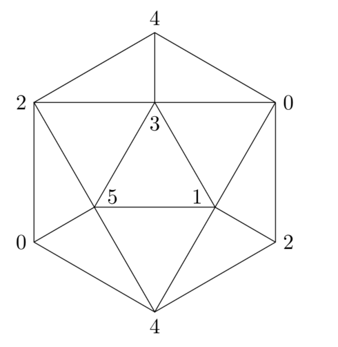
[1]:
rp2 = (
    (0,),
    (1,), (0,1),
    (2,), (0,2), (1,2), (0,1,2),
    (3,), (0,3), (1,3), (0,1,3), (2,3),
    (4,), (0,4), (1,4), (2,4), (1,2,4), (3,4), (0,3,4), (2,3,4),
    (5,), (0,5), (1,5), (2,5), (0,2,5), (3,5), (1,3,5), (2,3,5), (4,5), (0,4,5), (1,4,5)
    )

filtration = rp2
maxdim = max(map(len, filtration)) - 1
m = len(filtration) - 1
What will be computed
Relative cohomology
We will consider the persistent relative cohomology of \(X\)
as a persistence module.
Regular barcode
For \(i < j \in \{-1,\dots,m\}\) let \(X_{ij}\) be the unique composition \(H^\bullet(X, X_{i}) \leftarrow H^\bullet(X, X_{j})\) with the convention \(X_{-1} = \emptyset\). The barcode of this persistence module is the multiset
defined by the property
Steenrod barcode
Since the cohomology operation \(Sq^k\) is natural, we obtain an endomorphism of persistent relative cohomology
\begin{align*} &H^\bullet(X) \leftarrow \cdots \leftarrow H^\bullet(X, X_{m}) \\ & {\tiny Sq^k} \uparrow \kern 2.5cm {\tiny Sq^k} \uparrow\\ &H^\bullet(X) \leftarrow \cdots \leftarrow H^\bullet(X, X_{m}). \end{align*}
The \(Sq^k\)-barcode of \(X\) is the barcode of the image persistent module of this endomorphism.
Let us now compute these invariants using steenroder. We remark that since there is a compilation step required, the first time this function is run takes a bit long.
[2]:
from steenroder import barcodes

k = 1
barcode, steenrod_barcode = barcodes(k, filtration)
For each dimension d each of these is a 2D int array of shape (n_bars, 2) containing the bars of persistent relative cohomology and of the image of \(Sq^k\) in degree d. Let us inspect this output.
[3]:
print('Persistent relative cohomology:')

print('Regular barcode:')
for d in range(maxdim + 1):
    print(f'dim {d}:{list(map(list, barcode[d]))}')

print(f'Sq^{k}-barcode:')
for d in range(maxdim + 1):
    print(f'dim {d}:{steenrod_barcode[d]}')
Persistent relative cohomology:
Regular barcode:
dim 0:[[-1, 0]]
dim 1:[[20, 21], [12, 13], [-1, 11], [7, 8], [3, 4], [1, 2]]
dim 2:[[-1, 30], [28, 29], [22, 27], [25, 26], [23, 24], [14, 19], [17, 18], [15, 16], [9, 10], [5, 6]]
Sq^1-barcode:
dim 0:[]
dim 1:[]
dim 2:[[-1 11]]
There are three infinite bars in the regular barcode [-1,0] in deg 0, [-1,11] in deg 1, [-1,30] in deg 2. Additionally, there is one \(Sq^1\)-bar [-1,11] in deg 2. This \(Sq^1\)-bar witnesses in the persistent context the non-trivial relationship \(Sq^1 [\alpha_1] = [\alpha_2]\) between the degree 1 and 2 generators of the cohomology of \(\mathbb R P^2\).
How this is computed
We will now describe an effective computation of the \(Sq^k\)-barcode of persistent relative cohomology bulding on the computation of regular barcodes and persistent cocycle representatives. We refer to the notebook barcode where more details about this computation are given. Recall that the \(Sq^k\)-barcode is by definition the barcode of the image persistent module of the endomorphism \(Sq^k\).
The \(R = D^\perp V\) decomposition
Let \(D\) be the boundary matrix of the filtration with respect to the ordered basis of simplices and \(D^\perp\) its antitransposed:
where \(\overline j = m-j\) for \(j \in \{0,\dots,m\}\).
Let us consider the unique decomposition \(R = D^\perp V\) where \(V\) is an invertible upper triangular matrix and \(R\) is reduced, i.e., no two columns have the same pivot row.
The regular barcode
Denoting the \(i\)-th column of \(R\) by \(R_{i}\) where \(i \in \{0,\dots,m\}\), let
There exists a canonical bijection between the union of \(N\) and \(E\) and the persistence relative cohomology barcode of the filtration given by
\begin{align*} N \ni j &\mapsto \Big[\, \overline j, \overline{\mathrm{pivot}\,R_j}\, \Big] \in Bar^{\dim(j)+1}_X \\ E \ni j &\mapsto \big[\! -1, \overline j \,\big] \in Bar^{\dim(j)}_X \end{align*}
Representatives
Additionally, a persistent cocycle representative for each bar is given by \begin{equation*} [i,j] \mapsto \begin{cases} V_{\overline j}, & i = -1, \\ R_{\overline i}, & i \neq -1. \end{cases} \end{equation*} More specifically, a basis for \(H^\bullet(X, X_{\overline j-1})\) thought of as a subspace in the direct sum
is given by the set of cochains corresponding to the vectors in the union of
and a basis for \(\mathrm{img} \delta\) is given by
and a basis of coboundaries in \(C^\bullet(X, X_{\overline j})\) corresponds to non-zero vectors in
\begin{equation*} \{R_i\ |\ i \in N,\, i \leq j\}. \end{equation*}
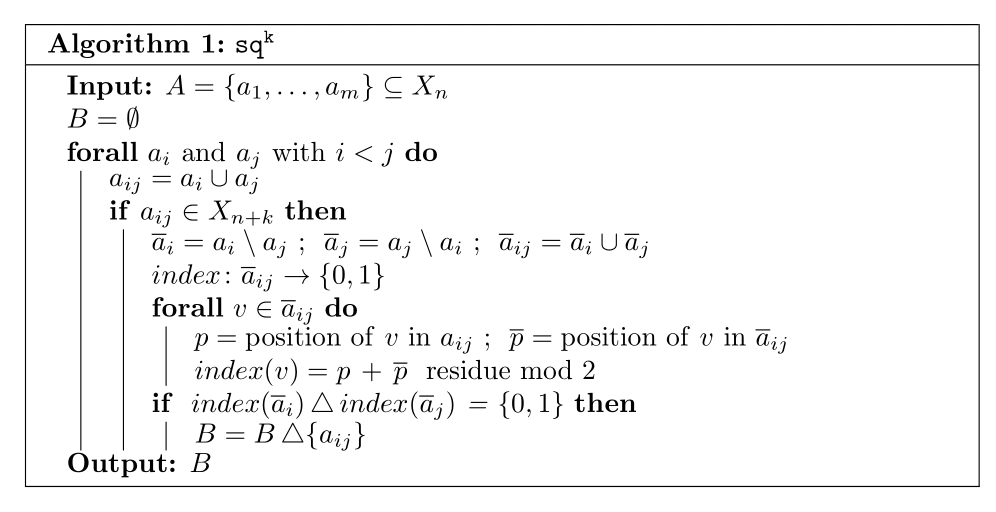
Steenrod representatives
Given vector \(v\) corresponding to a cocycle \(\alpha\), let \(\mathtt{sq^k}(v)\) be the vector correponding to cocycle representative of \(Sq^k \big( [\alpha] \big)\). For example, the one obtained using the following pseudo-code, where \(A\) is the support of \(\alpha\).
Steenrod matrix
Identifying a vector with the support of its associated cochain, define \(Q^k\) to be the matrix whose columns are given by
\begin{equation*} Q^k_i = \begin{cases} \mathtt{sq^k}(V_i), & i \in E, \\ \mathtt{sq^k}(R_j), & i = pivot(R_j), \\ 0, & otherwise. \end{cases} \end{equation*}
Reduction
Given \(R\) and \(Q^k\), we denote by \(R_{\le j}\) and \(Q^k_{\le j}\) the submatrices containing all columns with indices less than or equal to \(j\), and \(R_{\le j} \mid Q^k_{\le j}\) the matrix obtained by concatenating their columns. With this notation the following pseudo-code computes the \(k\)-Steenrod barcode of the filtration.
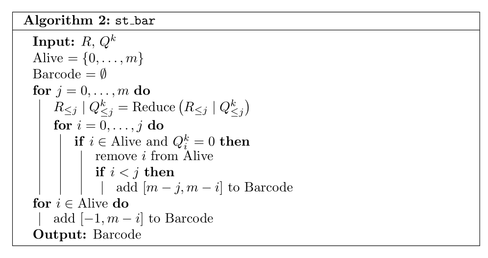
Intuitively, the step from \(j-1\) to \(j\) either adds a new non-zero coboundary \(R_j\) (which implies \(Q^k_j = 0\)) or the image \(Q^k_j\) of a persistent cocycle generator (which implies \(R_j=0\)). In either case, we need to reduce with respect to the subspace of coboundaries, generated by \(R_{\leq j}\), the image of \(Sq^k\), which is generated by \(Q^k_{\leq j}\). This process is done keeping track of when columns in \(Q^k\) become zero and extracting from this information the \(Sq^k\)-barcode of the filtration.
Using steenroder
Let us start by using the following functions explained in more detail in the notebook barcode.
[4]:
from steenroder import sort_filtration_by_dim, compute_reduced_triangular, compute_barcode_and_coho_reps

filtration_by_dim = sort_filtration_by_dim(filtration)
spx2idx, idxs, reduced, triangular = compute_reduced_triangular(filtration_by_dim)
barcode, coho_reps = compute_barcode_and_coho_reps(idxs, reduced, triangular)
Using an implementation of Algorithm 1, steenroder constructs the Steenrod matrix using the method compute_steenrod_matrix. Its output is a list of numba.typed.List, one list per simplex dimension. Explicitly, steenrod_matrix[d][j] entry is the result of computing the Steenrod square of coho_reps[d][j].
Since we are studying \(Sq^k\big([\alpha]\big)\) for \(k=1\) we concentarte on classes \([\alpha]\) of degree \(1\) since \(Sq^1\big([\alpha]\big) = 0\) otherwise.
[5]:
from steenroder import compute_steenrod_matrix

k = 1
steenrod_matrix = compute_steenrod_matrix(k, coho_reps, filtration_by_dim, spx2idx)

d = 1
print(f'Bar     : Cocycle --> Sq^{k}-cocycle:')
for bar, coho_rep, st_coho_rep in zip(barcode[d], coho_reps[d], steenrod_matrix[d+1]):
    cocycle = []
    for p in coho_rep:
        cocycle.append(filtration[idxs[d][p]])
    st_cocycle = []
    for p in st_coho_rep:
        st_cocycle.append(filtration[idxs[d+1][p]])
    print(f'{str(bar): <7} : {set(cocycle)} --> {st_cocycle}')
Bar     : Cocycle --> Sq^1-cocycle:
[20 21] : {(1, 5), (4, 5), (0, 5), (2, 5), (3, 5)} --> []
[12 13] : {(2, 4), (0, 4), (3, 4), (1, 4), (4, 5)} --> [(0, 4, 5), (1, 4, 5)]
[-1 11] : {(2, 4), (1, 5), (1, 4), (2, 3), (3, 5)} --> [(2, 3, 5)]
[7 8]   : {(3, 4), (0, 3), (2, 3), (1, 3), (3, 5)} --> [(0, 3, 4), (2, 3, 4), (1, 3, 5), (2, 3, 5)]
[3 4]   : {(2, 4), (1, 2), (2, 3), (0, 2), (2, 5)} --> [(1, 2, 4), (0, 2, 5)]
[1 2]   : {(0, 1), (1, 2), (1, 5), (1, 4), (1, 3)} --> [(0, 1, 2), (0, 1, 3)]
We will compare these representatives with those produced by a more explicit implementation of Algorithm 1.
[6]:
from itertools import combinations

def sq(k, cocycle, filtration):
    '''Return a cocycle representative of the image of Sq^k applied to the class represented by the given cocycle'''
    st_cocycle = set()
    for pair in combinations(cocycle, 2):
        a, b = set(pair[0]), set(pair[1])
        if (len(a.union(b)) == len(a) + k and
                tuple(sorted(a.union(b))) in filtration):
            a_bar, b_bar = a.difference(b), b.difference(a)
            index = dict()
            for v in a_bar.union(b_bar):
                pos = sorted(a.union(b)).index(v)
                pos_bar = sorted(a_bar.union(b_bar)).index(v)
                index[v] = (pos + pos_bar) % 2
            index_a = {index[v] for v in a_bar}
            index_b = {index[w] for w in b_bar}
            if (index_a == {0} and index_b == {1}
                    or index_a == {1} and index_b == {0}):
                u = sorted(a.union(b))
                st_cocycle ^= {tuple(u)}
    return st_cocycle
Let us not compute cocycle representatives generating the image of \(Sq^k\).
[7]:
d = 1
print(f'Cocycle --> Sq^{k}-cocycle:')
for coho_rep in coho_reps[d]:
    cocycle = []
    for p in coho_rep:
        cocycle.append(filtration[idxs[d][p]])
    st_cocycle = sq(k, cocycle, filtration)
    print(f'{set(cocycle)} --> {st_cocycle}')
Cocycle --> Sq^1-cocycle:
{(1, 5), (4, 5), (0, 5), (2, 5), (3, 5)} --> set()
{(2, 4), (0, 4), (3, 4), (1, 4), (4, 5)} --> {(1, 4, 5), (0, 4, 5)}
{(2, 4), (1, 5), (1, 4), (2, 3), (3, 5)} --> {(2, 3, 5)}
{(3, 4), (0, 3), (2, 3), (1, 3), (3, 5)} --> {(0, 3, 4), (2, 3, 4), (2, 3, 5), (1, 3, 5)}
{(2, 4), (1, 2), (2, 3), (0, 2), (2, 5)} --> {(1, 2, 4), (0, 2, 5)}
{(0, 1), (1, 2), (1, 5), (1, 4), (1, 3)} --> {(0, 1, 2), (0, 1, 3)}
It is carried through in compute_steenrod_barcode, whose output is the \(Sq^k\)-barcode of the filtration.
[8]:
from steenroder import compute_steenrod_barcode

dd = d + k
steenrod_barcode = compute_steenrod_barcode(k, steenrod_matrix, idxs, reduced, barcode)
steenrod_barcode[dd]
[8]:
array([[-1, 11]])
We will compare this output to an explicit construction obtained by implementing the above algorithms. Let us start by representing the matrix \(Q\) and \(R\) as instances of np.array. Recall that steenroder indexes everything with respect to the order of the original filtration, so we need to apply the transformation \((p,q) \mapsto (m-p, m-q)\) to the entries of the (sparse) matrices it produces.
[9]:
import numpy as np

antiQ = np.zeros((m+1,m+1), dtype=int)
for d in range(maxdim-k+1):
    for bar, col in zip(barcode[d], steenrod_matrix[d+k]):
        for p in col:
            antiQ[idxs[d+k][p], bar[1]] = 1
Q = np.flip(antiQ, [0,1])

antiR = np.zeros((m+1,m+1), dtype=int)
for d in range(maxdim+1):
    for i, col in enumerate(reduced[d]):
        for j in col:
            antiR[idxs[d+1][j], idxs[d][i]] = 1
R = np.flip(antiR, [0,1])
Before introducing an implementation of Algorithm 2 we need some auxiliary functions:
[10]:
def pivot(column):
    """Returns the index of the largest non-zero entry of the column or None if all entries are 0"""
    try:
        return max(column.nonzero()[0])
    except ValueError:
        return None

def reduce_vector(reduced, column):
    """Reduces a column with respect to a reduced matrix with the same number of rows"""
    num_col = reduced.shape[1]
    i = -1
    while i >= -num_col:
        if not np.any(column):
            break
        else:
            piv_v = pivot(column)
            piv_i = pivot(reduced[:, i])

            if piv_i == piv_v:
                column[:, 0] = np.logical_xor(reduced[:, i], column[:, 0])
                i = 0
            i -= 1

def reduce_matrix(reduced, matrix):
    """Reduces a matrix with respect to a reduced matrix with the same number of rows"""
    num_vector = matrix.shape[1]
    reducing = reduced.copy()

    for i in range(num_vector):
        reduce_vector(reducing, matrix[:, i:i+1])
        reducing = np.concatenate([reducing, matrix[:, i:i+1]], axis=1)
We now define a function implementing Algorithm 2. Using it we obtain the same Steenrod barcode as the one produced by steenroder.
[11]:
def get_steenrod_barcode(R, Q):
    """Returns the Steenrod barcodes implementing Algorithm 2"""
    m = R.shape[1]-1
    alive = {i: True for i in range(m)}
    steenrod_barcode = []
    for j in range(m):
        reduce_matrix(R[:,:j+1], Q[:,:j+1])
        for i in range(j+1):
            if alive[i] and not np.any(Q[:,i]):
                alive[i] = False
                if j > i:
                    steenrod_barcode.append([m-j, m-i])
    steenrod_barcode += [[-1,m-i] for i in alive if alive[i]]
    return steenrod_barcode

get_steenrod_barcode(R, Q)
[11]:
[[-1, 11]]
duality and truncations