The regular barcode of persistent relative cohomology
In this notebook we illustrate the use of steenroder for the computation of the regular barcode of persistent relative cohomology with mod 2 coefficients. The filtered simplicial complex \(X\) that we consider is a model for the circle
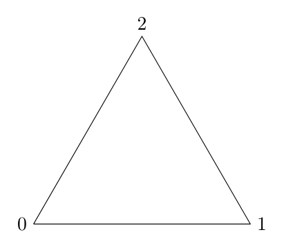
given by the following tuple of tuple of int:
[1]:
circle = (
    (0,),
    (1,), (0,1),
    (2,), (1,2), (0,2)
    )

filtration = circle
maxdim = max([len(spx)-1 for spx in filtration])
m = len(filtration)-1
Relative cohomology
We will consider the persistent relative cohomology of \(X\)
as a persistence module.
Its regular barcode
For \(i < j \in \{-1,\dots,m\}\) let \(X_{ij}\) be the unique composition \(H^\bullet(X, X_{i}) \leftarrow H^\bullet(X, X_{j})\) with the convention \(X_{-1} = \emptyset\). The barcode of this persistence module is the multiset
defined by the property
[2]:
from steenroder import barcodes

barcode, steenrod_barcode = barcodes(0, filtration)

print(f'Barcode of persistent relative cohomology:')
for d in range(maxdim + 1):
    print(f'dim {d}: \n{barcode[d]}')
Barcode of persistent relative cohomology:
dim 0:
[[-1  0]]
dim 1:
[[-1  5]
 [ 3  4]
 [ 1  2]]
How this is computed
Boundary matrix
Order the simplices \(a_0 < a_1 < \dots < a_m\) of \(X\) so that \(X_k = \{a_i \mid i \leq k\}\). Consider the matrix \(D\) representing the boundary map \(\partial \colon C_\bullet(X;\mathbb{F}_2) \to C_{\bullet-1}(X;\mathbb{F}_2)\) with respect to the (ordered) basis determined by the (ordered) simplices. Explicitly,
Notice that the submatrix \(D_{\leq j \leq j}\) represents the boundary of \(C_\bullet(X_j;\mathbb F_2)\) for every \(k \in \{0,\dots,m\}\).
Anti-transpose
We will consider the antitranspose \(D^\perp\) of the boundary matrix \(D\). It is defined for every \(p,q \in \{0, \dots, m\}\) by
where \(\overline j = m-j\) for \(j \in \{0, \dots, m\}\)
For any \(j \in \{0,\dots,m\}\) the submatrix \(D^\perp_{\leq j, \leq j}\) represents the coboundary map \(\delta \colon C^\bullet(X, X_{\overline j-1}; \mathbb{F}_2) \to C^{\bullet+1}(X, X_{\overline j-1}; \mathbb{F}_2)\) with respect to the (ordered) dual basis \(a_m^\bullet < \dots < a_{m-j}^\bullet\).
The \(R = D^\perp V\) decomposition
Here \(V\) is an invertible upper triangular matrix and \(R\) is reduced, i.e., no two columns have the same pivot row.
Denoting the \(i\)-th column of \(R\) by \(R_{i}\) where \(i \in \{0,\dots,m\}\), let
The regular barcode
There exists a canonical bijection between the union of \(N\) and \(E\) and the persistence relative cohomology barcode of the filtration given by
\begin{align*} N \ni j &\mapsto \Big[\, \overline j, \overline{\mathrm{pivot}\,R_j}\, \Big] \in Bar^{\dim(a_j)+1}_X \\ E \ni j &\mapsto \big[\! -1, \overline j \, \big] \in Bar^{\dim(a_j)}_X \end{align*}
Representatives
Additionally, a persistent cocycle representative is given by \begin{equation*} [i,j] \mapsto \begin{cases} V_{\overline j}, & i = -1, \\ R_{\overline i}, & i \neq -1. \end{cases} \end{equation*}
Using steenroder
Splitting by dimension
In steenroder all computations are done dimension by dimension. We start by splitting the filtration into collection of simplices of the same dimension.
[3]:
from steenroder import sort_filtration_by_dim

filtration_by_dim = sort_filtration_by_dim(filtration)
The output of sort_filtration_by_dim is as follows:
For each dimension d, a list of 2 aligned int arrays: the first is a 1D array containing the (ordered) positional indices of all d-dimensional simplices in filtration; the second is a 2D array whose i-th row is the (sorted) collection of vertices defining the i-th d-dimensional simplex.
[4]:
print(f'Simplices:')
for d in range(maxdim + 1):
    positions, simplices = filtration_by_dim[d]
    print(f'dim {d}:\n{simplices}\nin positions {positions}.')
Simplices:
dim 0:
[[0]
 [1]
 [2]]
in positions [0 1 3].
dim 1:
[[0 1]
 [1 2]
 [0 2]]
in positions [2 4 5].
A note on anti-transposition
The anti-transposition operation \((-)^\perp\) is determined by composing the usual trnasposition
and the horizontal and vertical flips
We remark that
for any pair of square matrices \(M\) and \(N\).
The \(R = D^\perp V\) decomposition
To compute the matrices \(R\) and \(V\) in the decomposition \(R = D^\perp V\) steenroder uses the method compute_reduced_triangular. It actually produces \(R^\mathrm{A}\) and \(V^\mathrm{A}\). More precisely, the output reduced is a tuple of numba.typed.List with reduced[d] the d-dimensional part of \(R^\mathrm{A}\). More explicitly, for an integer \(j\) we have that an integer \(i\) is in the tuple reduced[d][j] if and only if
\(R^\mathrm{A}_{ij} = 1\). Similarly triangular[d] is the d-dimensional part of the \(V^\mathrm{A}\). There are also two other auxiliary outputs that will be discussed later, these are spx2idx and idxs.
[5]:
from steenroder import compute_reduced_triangular

spx2idx, idxs, reduced, triangular = compute_reduced_triangular(filtration_by_dim)
We will verify for our running example that \(R = D^\perp V\) by checking that the coboundary \(D^\mathrm{T}\) of this filtration is equal to \(R^\mathrm{A} U^\mathrm{A}\) where \(U\) is the inverse of \(V\).
Let us start by contructing the coboundary matrix \(D^\mathrm{T}\).
[6]:
import numpy as np

coboundary = np.zeros((m+1,m+1), dtype=int)
for j, x in enumerate(filtration):
    for i, y in enumerate(filtration):
        if len(x)+1 == len(y) and set(x).issubset(set(y)):
            coboundary[i,j] = 1
print(f'D^T =\n{coboundary}')
D^T =
[[0 0 0 0 0 0]
 [0 0 0 0 0 0]
 [1 1 0 0 0 0]
 [0 0 0 0 0 0]
 [0 1 0 1 0 0]
 [1 0 0 1 0 0]]
We now represent \(R^{\mathrm{A}}\) and \(V^{\mathrm{A}}\) as instances of np.array, compute \(U^{\mathrm{A}}\) and verify that \(U^{\mathrm{A}} R^{\mathrm{A}}\) is equal to \(D^{\mathrm{T}}\) as claimed.
[7]:
def to_array(matrix, e=0):
    """Transforms reduced (e=1) and triangular (e=0) to numpy arrays"""
    array = np.zeros((m+1,m+1), dtype=int)
    for d in range(maxdim+1):
        for i, col in enumerate(matrix[d]):
            for j in col:
                array[idxs[d+e][j], idxs[d][i]] = 1
    return array

antiR, antiV = to_array(reduced, e=1), to_array(triangular, e=0)
antiU = np.array(np.linalg.inv(antiV), dtype=int)
product = np.matmul(antiR, antiU) % 2
print(f'D^T = R^AU^A: {(coboundary == product).all()}')
D^T = R^AU^A: True
Regular barcode and persistent cocycle representatives
[8]:
from steenroder import compute_barcode_and_coho_reps

barcode, coho_reps = compute_barcode_and_coho_reps(idxs, reduced, triangular)
For every d we have that barcode[d] is a 2D int array of shape (n_bars, 2) containing the birth (entry 1) and death (entry 0) indices of persistent relative cohomology classes in degree d.
[9]:
for d in range(maxdim+1):
    print(f'The barcode in dim {d}:\n{barcode[d]}')
The barcode in dim 0:
[[-1  0]]
The barcode in dim 1:
[[-1  5]
 [ 3  4]
 [ 1  2]]
We will compare this barcode with its description as
\begin{align*} N \ni j &\mapsto \Big[\, \overline j, \overline{\mathrm{pivot}\,R_j} \, \Big] \in Bar_{{\dim(j)+1}}^{\mathrm{fin}} \\ E \ni j &\mapsto \big[\! -1, \overline j \, \big] \in Bar_{\dim(j)}^{\mathrm{inf}} \end{align*} where
Let us start by obtaining \(R\) from \(R^{\mathrm{A}}\).
[10]:
R = np.flip(antiR, [0,1])
print(f'R =\n{R}')
R =
[[0 0 1 0 0 0]
 [0 0 1 0 1 0]
 [0 0 0 0 0 0]
 [0 0 0 0 1 0]
 [0 0 0 0 0 0]
 [0 0 0 0 0 0]]
We can not construct the sets \(P\), \(N\) and \(E\).
[11]:
def pivot(column):
    try:
        return max(column.nonzero()[0])
    except ValueError:
        pass

P, N, E = [], [], []
for i, col in enumerate(R.T):
    if pivot(col):
        N.append(i)
        E.remove(pivot(col))
    else:
        P.append(i)
        E.append(i)

print(f'P = {P}\nN = {N}\nE = {E}')
P = [0, 1, 3, 5]
N = [2, 4]
E = [0, 5]
Finally we deduce the barcode from these.
[12]:
bcode = [[] for d in range(maxdim+1)]

for j in N:
    d = len(filtration[m-j])
    bcode[d].append([m-j, m-pivot(R[:,j])])

for j in E:
    d = len(filtration[m-j])-1
    bcode[d].append([-1, m-j])

for d in range(maxdim+1):
    print(f'The barcode in dim {d}:\n{bcode[d]}')
The barcode in dim 0:
[[-1, 0]]
The barcode in dim 1:
[[3, 4], [1, 2], [-1, 5]]
Let us now consider the other output coho_reps[d][k]. It is a list of positional indices, relative to the d-dimensional portion of the filtration, representing the bar barcode[d][k] for every k.
To express these representatives in terms of cochains, we use that idxs[d] is an int array containing the (ordered) positional indices of all d-dimensional simplices in the filtration.
[13]:
for d in range(maxdim+1):
    for bar, rel_positions in zip(barcode[d], coho_reps[d]):
        coho_rep = []
        for p in rel_positions:
            coho_rep.append(filtration[idxs[d][p]])
        print(f"{str(bar): <7} rep. by {coho_rep}")
[-1  0] rep. by [(0,), (1,), (2,)]
[-1  5] rep. by [(0, 2)]
[3 4]   rep. by [(1, 2), (0, 2)]
[1 2]   rep. by [(0, 1), (1, 2)]
We will now compare these representatives to their description as \begin{equation*} [i,j] \mapsto \begin{cases} V_{\bar j}, & i = -1, \\ R_{\bar i}, & i \neq -1. \end{cases} \end{equation*}
[14]:
V = np.flip(antiV, [0,1])

for d in range(maxdim+1):
    for bar in barcode[d]:
        i,j = bar
        c_rep = []
        if i == -1:
            nonzeros = np.nonzero(V[:,m-j])[0]
        else:
            nonzeros = np.nonzero(R[:,m-i])[0]
        for p in nonzeros:
            c_rep.append(filtration[m-p])
        print(f'{str(bar): <7} rep. by {c_rep}')
[-1  0] rep. by [(2,), (1,), (0,)]
[-1  5] rep. by [(0, 2)]
[3 4]   rep. by [(0, 2), (1, 2)]
[1 2]   rep. by [(1, 2), (0, 1)]
To-Do
Explain duality between persistent relative cohomology and persistent homology.